Frequency Domain Adaptive Noise Cancellation
August 8, 2025
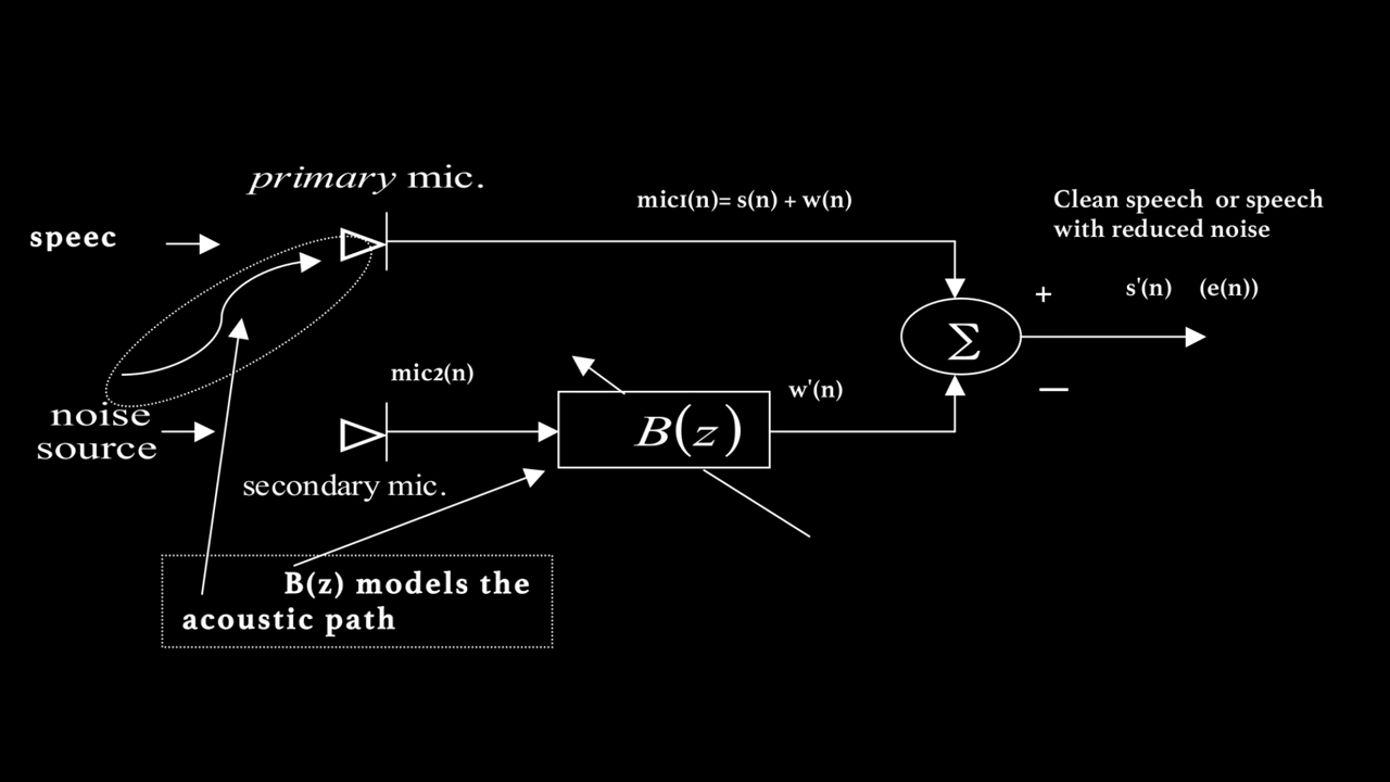 Figure 1: Adapative Noise Canceller
Overview
An adaptive filter is a self-adjusting digital filter that automatically adjusts its coefficients using algorithms like the Least Mean Squares to minimize error and model a desired signal in real time. Unlike fixed filters, it continuously adapts to changing input conditions, making it common for applications like noise cancellation, echo suppression, system identification, and signal prediction. In this project an adaptive filter using the NLMS algorithm is used in an attempt to cancel out noise from a signal that contains speech+background noise.
Model
Figure 1 shows the system diagram of the adaptive noise canceller that will be modeled. The system uses two microphones:
- Mic1 is placed near the speaker. It captures the clean speech but also contains unwanted background noise.
- Mic2 is placed farther from the speaker and closer to the noise source.
The goal is to use the noise captured by Mic2 to remove the noise present in Mic1, producing a cleaner speech signal.
However, the noise in Mic1 is not identical to the noise in Mic2. Due to the acoustic path between the noise source and Mic1, the noise in Mic1 may include reflections, delays, and other distortions. This means we cannot just subtract Mic2’s signal from Mic1’s signal.
To address this, an FIR filter $ B(z) $ is used to model how the noise from Mic2 appears at Mic1. The coefficients of $ B(z) $ are continuously updated using the Normalized Least Mean Squares (NLMS) algorithm.
The primary microphone signal is:
$$ s(n) + w(n) $$
where:
- $ n $ is the time index,
- $ s(n) $ is the clean speech signal,
- $ w(n) $ is the noise at Mic1.
After noise cancellation, the output signal is:
$$ s(n) + w(n) - w'(n) $$
where $ w'(n) $ is the estimated noise obtained from filtering Mic2’s signal through $ B(z) $.
Algorithm
Read audio from the primary and secondary microphones.
Take a frame of size $N$ to analyze and apply a window (e.g., Hanning) to reduce spectral leakage.
Take the DFT:
- Use zero-padding to increase DFT frequency resolution.
- Apply zero-phase windowing by circularly shifting the frame so its center is at index 0, preventing phase offsets. For real, symmetric windows $w[n]$, the Fourier transform will be real-valued, avoiding unwanted phase changes in $X$.
Estimate noise in the frequency domain:
$$ Y = B \cdot X $$ where $B$ is the adaptive filter and $X$ is Mic2’s spectrum.Subtract noise from the primary mic:
$$ E = D - Y $$ where $D$ is Mic1’s spectrum, and $E$ is the error (cleaned signal).Update filter coefficients using Normalized LMS:
$$ B \mathrel{+}= \frac{2 \mu \cdot \mathrm{conj}(X) \cdot E}{|X|^2 + \varepsilon} $$ where $B$ are the filter coefficients, $X$ is Mic2's spectrum, $E$ is the error signal, $\mu$ is the step size, and $\varepsilon$ is a small constant for numerical stability.Inverse FFT and overlap-add to reconstruct the time-domain signal.
Repeat steps 2–7 until the end of the audio (advancing frames by hop size).
Normalize and output both the clean signal and the separated noise.
Parameters
Frame Size ($N$)
Determines the length of each analysis frame.
Hop Size (hop_size)
Specifies the number of samples to advance to the next frame (i.e., the frame shift).
Step Size ($\mu$)
Controls the adaptation rate of the filter coefficients:
- Small $\mu$: Adaptation is slow but stable. This is safer but may cause the filter to react sluggishly to changes in the noise environment.
- Large $\mu$: Adaptation is fast, allowing quick response to changes. However, it may cause instability, distortion, or artifacts such as “pre-echo” or “post-echo” when the filter overreacts to sudden transitions.
Epsilon ($\epsilon$)
A small constant added to ensure numerical stability during calculations, preventing division by zero or very small denominators.
Window ($window$)
The type of window applied to each frame to reduce spectral leakage.
Filter ($B$)
The initial filter coefficients that will be adapted over time.
Code
import numpy as np
import soundfile as sf
from scipy.fft import fft, ifft
from scipy.signal.windows import hann
import matplotlib.pyplot as plt
# === Helper Function ===
def moving_average(x, w):
    return np.convolve(x, np.ones(w)/w, mode='valid')

# === Load signals ===
mic1, fs = sf.read("mic1_noise.wav")  # speech + noise
mic2, _  = sf.read("mic2_noise.wav")  # noise reference

# === Parameters ===
N = 512            # FFT/frame size
hop_size = N // 2   # 50% overlap
mu = 0.0015         # Step size (smaller = more stable)
eps = 1e-6         # For numerical stability
window = hann(N)
B = np.zeros(N, dtype=complex)

# Trim to equal length
length = min(len(mic1), len(mic2))
mic1 = mic1[:length]
mic2 = mic2[:length]

# === Init ===
output = np.zeros(length + N)
weight = np.zeros(length + N)
error_db = []
snr_db = []

# === Adaptive Loop ===
for i in range(0, length - N, hop_size):
    frame_i = slice(i, i + N)

    # Window a frame of the input from mic1 and mic2
    d = mic1[frame_i] * window
    x = mic2[frame_i] * window

    # Calculate the FFT
    D = fft(d)
    X = fft(x)

    # Estimate noise in the frequency domain (Y)
    Y = B * X

    # Subtract the noise from the primary mic
    E = D - Y

    # Update filter coefficients using Normalized LMS
    # study lms and conjugation and how coeficients are adjusted.
    B += 2 * mu * np.conj(X) * E / (np.abs(X)**2 + eps)

    # IFFT to time domain
    e = np.real(ifft(E)) * window

    # Overlap-add
    output[i:i+N] += e
    weight[i:i+N] += window**2

    # Error and SNR calculations
    error_power = np.sum(np.abs(E)**2)
    signal_power = np.sum(np.abs(D)**2)
    error_db.append(10 * np.log10(error_power + eps))
    snr_db.append(10 * np.log10(signal_power / (error_power + eps)))

# === Normalize output ===
nonzero = weight > 1e-6
output[nonzero] /= weight[nonzero]
output = output[:length]

peak = np.max(np.abs(output))
if peak > 1e-6:
    output /= peak

# === Save result ===
np.save('B.npy', B) # Final filter coefficients
sf.write("output.wav", output, fs)

# === Plot convergence curves ===
plt.figure(figsize=(10, 5))

# Error convergence
plt.subplot(2, 1, 1)
plt.plot(moving_average(error_db, w=64))
plt.title("Convergence Curve (Error Power in dB)")
plt.xlabel("Frame Index")
plt.ylabel("Error Power (dB)")
plt.grid(True)

# SNR improvement
plt.subplot(2, 1, 2)
plt.plot(moving_average(snr_db, w=64))
plt.title("SNR Over Time")
plt.xlabel("Frame Index")
plt.ylabel("SNR (dB)")
plt.grid(True)

plt.tight_layout()
plt.show()
Output
Audio Samples
Input Audio from Microphone 1
Input Audio from Microphone 2
Output Audio After 1 Pass
Output Audio After 2 Pass
You can hear the adaptive noise filter slowly removing the noise in the output audio. With the filter coefficients $B(z)$ initialized from the first pass, the noise cancellation is much more effective.
Performance Evaluation
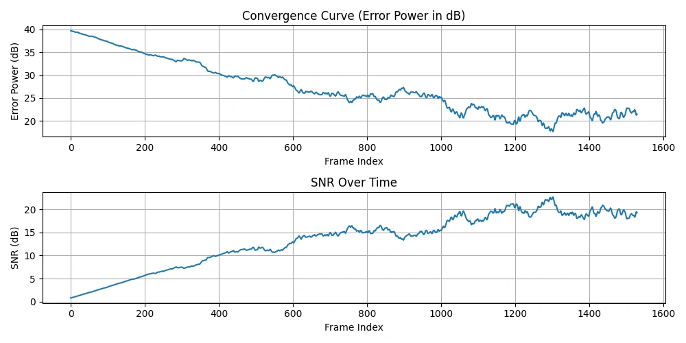 Figure 2: Plot of Convergence Curve and SNR Over Time
Convergence Curve (Error Power in dB)
$$ \mathrm{errorPower} = \sum_{n=1}^{N} |E(n)|^2 $$
$$ \text{Error Power (dB)} = 10 \log_{10}\bigl(\mathrm{errorPower} + \varepsilon\bigr) $$
This curve shows how the error power (residual noise energy) decreases over time as the adaptive filter learns to cancel noise.
Signal-to-Noise Ratio (SNR) per Frame
$$ \mathrm{signalPower} = \sum_{n=1}^{N} |D(n)|^2 $$
$$ \mathrm{errorPower} = \sum_{n=1}^{N} |E(n)|^2 $$
$$ \mathrm{SNR} = 10 \log_{10} \left( \frac{\mathrm{signalPower}}{\mathrm{errorPower} + \varepsilon} \right) $$
where:
- Signal Power = $|D|^2$ (power of primary mic frame spectrum)
- Error Power = $|E|^2$ (power of residual noise after cancellation)
The SNR typically increases over time as the adaptive filter improves noise suppression.
Moving Average
Applying a moving average to these curves smooths out fluctuations, making overall trends easier to visualize.
- The error power convergence curve demonstrates how effectively noise energy is reduced (should decrease).
- The SNR curve shows improvement in signal clarity relative to noise (should increase).
This inverse relationship makes intuitive sense: as the filter better estimates noise and cancels it, the residual error power drops, and the SNR improves.
Summary of Key Concepts
The frequency components $B(k)$ represent the adaptive filter’s frequency response, illustrating how noise captured by the secondary microphone is modified to cancel noise present in the primary microphone. Increasing the FFT size $N$ improves frequency resolution and allows for more accurate noise modeling, which can lead to higher SNR values. However, a larger $N$ also results in increased latency and slower filter adaptation.
There is a direct relationship between the FFT size $N$ and the filter order: a larger FFT corresponds to a longer filter capable of modeling more complex acoustic paths and longer impulse responses. The step size $\mu$ governs the speed and stability of filter adaptation; smaller values yield slow but stable adaptation with minimal distortion, whereas larger values enable faster adaptation at the risk of introducing distortions and artifacts such as musical noise or pre/post-echo.
Generally, a higher SNR correlates with better perceived speech quality, although excessively aggressive noise cancellation can produce audible artifacts that degrade the listening experience. Minimizing the error signal $e(n)$ is crucial because it reflects how effectively the filter cancels noise, thereby enhancing speech clarity. To understand the time-domain behavior of the filter, one can compute the inverse FFT of $B(k)$, translating frequency-domain filter coefficients back into the filter’s impulse response.
Conclusion
The frequency-domain adaptive filter effectively cancels noise by modeling and subtracting the noise spectrum from the primary microphone’s signal. Utilizing frequency-domain processing brings computational efficiency, particularly for long FIR filters, by leveraging FFT algorithms. The Normalized LMS algorithm ensures stable adaptation by normalizing the step size according to the reference signal’s power, reducing the likelihood of divergence.
Choosing the step size $\mu$ involves a trade-off: a smaller $\mu$ slows convergence but ensures stability, while a larger $\mu$ accelerates adaptation but risks instability and audible artifacts. Applying windowing and zero-phase alignment techniques reduces spectral leakage and phase distortion, resulting in improved filter performance. Overlap-add reconstruction guarantees a smooth, continuous output signal without gaps or discontinuities.
Future improvements may include more advanced adaptation methods such as Recursive Least Squares (RLS), adaptive step size control, or deploying multi-microphone arrays for more robust noise modeling. While real-time implementation demands further optimization, this frequency-domain approach lays a strong foundation for adaptive noise cancellation in both offline and real-time digital signal processing applications.