Monophonic Audio-to-MIDI Converter: Onsets, Pitch, and Transcription
August 10, 2025
Overview
Converting audio into MIDI data is a fundamental task in music technology, enabling analysis, editing, and synthesis of performances. Unlike polyphonic audio detection—where multiple harmonies and overlapping notes complicate analysis—monophonic audio detection deals with simpler signals and can achieve a more accurate representation using signal processing techniques.
In this project, I focus on building a monophonic audio-to-MIDI converter: a system designed to transcribe melodies where only one note sounds at a time. The approach I take is to first detect the onset times in the melody. Then, each onset frame is analyzed to estimate its pitch. Finally, the MIDI representation is produced by combining the detected onset times and pitch information.
For this project, note velocity (how forcefully a note is played) and note offsets (when a note ends) are assigned fixed values.
Onset Detection
The first step is onset detection: determining the time when each note begins. Typically, a note’s articulation involves an onset, attack, and decay phase. For this project, I tested classic techniques such as energy-based thresholding and spectral flux on recordings of piano and oboe.
Parameters were adjusted depending on the instrument. For piano, onsets and attacks tend to be sharper and more distinct, while for oboe they are generally less prominent and more gradual. Although both energy-based thresholding and spectral flux provided usable results with sufficient parameter tuning, spectral flux ultimately yielded better and more reliable onset detection.
The figures below illustrate onset detection using spectral flux for piano and oboe, alongside corresponding audio samples with onset taps.
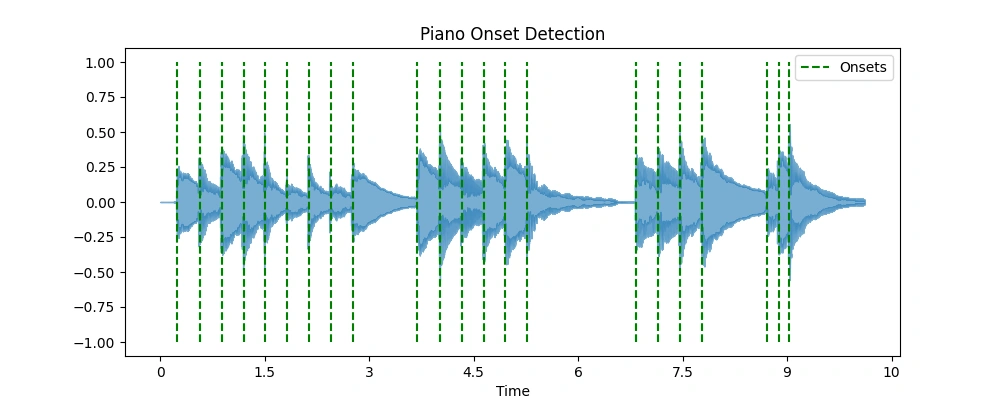 Piano Onset Detection Diagram
Input Audio from piano
 Oboe Onset Detection Diagram
Input Audio from oboe
Pitch Detection
Once the note start times are identified (from onset detection described in the previous section), the next step is to estimate the pitch. I implement and compare two well-known pitch detection algorithms: YIN and PYIN.
To evaluate these methods, I run the transcription pipeline on a single segment of a monophonic melody derived from the onset detection results. Below is a plot showing the difference function and cumulative mean normalized difference for the YIN algorithm.
 YIN Pitch Graph
YIN Algorithm
Step 1: Difference function
Given a frame of audio samples $x[n]$ of length $W$, the difference function $d(\tau)$ measures the squared difference between the signal and its delayed version by lag $\tau$:
$$ d(\tau) = \sum_{n=0}^{W-\tau-1} \big( x[n] - x[n+\tau] \big)^2 $$
Variables:
- $x[n]$: audio sample at index $n$
- $W$: total number of samples in the current frame (frame length)
- $\tau$: lag (delay) parameter, representing a candidate fundamental period
Step 2: Cumulative Mean Normalized Difference (CMND)
The cumulative mean normalized difference function $\text{cmnd}(\tau)$ normalizes $d(\tau)$ to improve robustness and make it easier to find the fundamental period:
$$ \text{cmnd}(\tau) = \begin{cases} 1, & \tau = 0, \ \dfrac{d(\tau)}{\frac{1}{\tau} \sum_{j=1}^{\tau} d(j)}, & \tau > 0 \end{cases} $$
Variables:
- $d(\tau)$: difference function from Step 1
- $\tau$: lag as above
Step 3: Absolute threshold to detect candidate fundamental period
Identify the smallest lag $\tau$ within the search range $[\tau_{\min}, \tau_{\max}]$ where the normalized difference is below a threshold, indicating a potential fundamental period:
$$ \text{Find smallest } \tau \in [\tau_{\min}, \tau_{\max}] \text{ such that } \text{cmnd}(\tau) < \text{threshold} $$
The search range bounds correspond to the expected frequency range:
$$ \tau_{\min} = \frac{f_s}{f_{\max}}, \quad \tau_{\max} = \frac{f_s}{f_{\min}} $$
Variables:
- $f_s$: sampling frequency of the audio signal (samples per second)
- $f_{\min}, f_{\max}$: minimum and maximum expected fundamental frequencies (Hz)
- $\text{threshold}$: a predefined cutoff (e.g., 0.1 to 0.2) to determine pitch candidates
Step 4: Estimated fundamental frequency
Once the candidate lag $\tau_{\text{est}}$ is found, the fundamental frequency estimate $f_0$ is:
$$ f_0 = \frac{f_s}{\tau_{\text{est}}} $$
Variables:
- $\tau_{\text{est}}$: lag selected as the estimated fundamental period
- $f_0$: estimated fundamental frequency (Hz)
The PYIN algorithm builds upon the classic YIN pitch detection method by taking a probabilistic approach that greatly improves pitch tracking accuracy. Instead of producing just a single pitch estimate per frame, PYIN generates multiple pitch candidates, each with an associated probability that reflects how well it matches the audio features within that frame, such as cumulative mean normalized difference (CMND) or energy.
What makes PYIN especially powerful is its ability to model the natural continuity of pitch over time. It incorporates transition probabilities that express how likely it is for the pitch to remain steady or change smoothly between consecutive frames — capturing the fact that sudden large jumps in pitch are rare in both speech and music.
To find the best overall pitch trajectory, PYIN uses the Viterbi algorithm, a dynamic programming method that efficiently searches for the most probable path through all candidate pitches across the entire audio sequence. This approach enforces temporal smoothness and reduces noise that can arise from analyzing frames independently.
Additionally, PYIN jointly estimates whether each frame is voiced or unvoiced, improving robustness in challenging acoustic conditions.
The combination of these elements results in cleaner, more natural pitch contours and more accurate voiced/unvoiced decisions. Below is a plot showing PYIN’s pitch candidates alongside the final pitch track—decoded via Viterbi—for the first segment of the oboe melody.
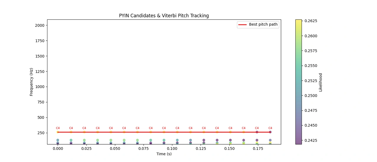 PYIN and Viterbi Pitch Tracking
Algorithm
Read the audio
Load the audio signal for processing.Compute the time-frequency representation
Use the Short-Time Fourier Transform (STFT) to convert the time-domain signal into a time-frequency representation. The STFT produces linear frequency bins, which are well suited for analyzing general spectral changes.Detect onsets using the magnitude spectrum
- Energy-based method: Calculate the energy difference between consecutive frames after circularly shifting the spectrum. Onsets are detected by comparing these differences against a threshold, typically set relative to the median energy level to adapt to varying signal dynamics.
- Spectral flux: Measure positive increases in spectral magnitude between frames. Onsets correspond to peaks in spectral flux, indicating new note attacks.
Estimate pitch at each detected onset
Analyze a short segment following each onset (usually 40–100 ms) to capture the note’s initial steady tone.- YIN algorithm: A time-domain method that uses autocorrelation differences to estimate the fundamental frequency accurately.
- PYIN algorithm: A probabilistic extension of YIN that offers smoother and more robust pitch tracking.
Save note data
Record the note’s start time (onset), estimated end time (such as the next onset or a fixed duration), and pitch frequency.- Velocity: Derived from the energy or amplitude at the onset to reflect note intensity; if unavailable, a fixed velocity can be assigned. Note velocity and offsets (note end times) are typically assigned fixed values for simplicity.
Output and synthesize MIDI
Convert the extracted note data into a MIDI file, and optionally synthesize it for audio playback.
Parameters
| Parameter | Description | Typical Values |
|---|---|---|
frame_length |
Window size for STFT or pitch analysis | 2048 samples |
hop_length |
Step size between analysis frames | 256 samples |
fmin |
Minimum frequency to detect pitch | ~27.5 Hz (A0) |
fmax |
Maximum frequency to detect pitch | ~4186 Hz (C8) |
delta |
Sensitivity threshold for spectral-flux onset detection | 0.12 (smaller = more sensitive) |
min_note_gap |
Minimum duration for a note | 0.05 seconds |
tentative_end_gap |
Gap before next onset to define note end | 0.02 seconds |
Example Code (Python)
import librosa
import numpy as np
import pretty_midi
from energyOnset import spectral_energy_onset_detect


def extract_midi_from_audio(audio_path, onset_method='spectral-flux',
                           pitch_method='yin'):
    # Parameters
    hop_length = 256
    frame_length = 2048
    fmin = librosa.note_to_hz('A0')  # Minimum pitch frequency
    fmax = librosa.note_to_hz('C7')  # Maximum pitch frequency

    # Load audio
    y, sr = librosa.load(audio_path)

    # Onset detection
    if onset_method == 'energy':
        onset_frames, onset_times = spectral_energy_onset_detect(y, sr)
    else:  # Default: spectral-flux method
        onset_frames = librosa.onset.onset_detect(
            y=y,
            sr=sr,
            hop_length=hop_length,
            pre_max=5,
            post_max=5,
            pre_avg=5,
            post_avg=5,
            delta=0.12,   # smaller delta for higher sensitivity
            wait=2
        )
        onset_times = librosa.frames_to_time(
            onset_frames, sr=sr, hop_length=hop_length)

    # Initialize PrettyMIDI and instrument
    pm = pretty_midi.PrettyMIDI()
    # Electric Piano by default
    melody_instr = pretty_midi.Instrument(program=4)
    # minimum duration of a note (seconds)
    min_note_gap = 0.05

    # Process each onset segment for pitch detection
    for i, onset_frame in enumerate(onset_frames):
        start_sample = onset_frame * hop_length
        end_sample = (onset_frames[i + 1] * hop_length
                      if i + 1 < len(onset_frames) else len(y))
        segment = y[start_sample:end_sample]

        # Skip segment if too short for pitch analysis
        if len(segment) < frame_length:
            continue

        # Pitch detection
        if pitch_method == 'pyin':
            f0_est, voiced_flag, _ = librosa.pyin(
                segment,
                fmin=fmin,
                fmax=fmax,
                sr=sr,
                frame_length=frame_length,
                hop_length=hop_length,
                fill_na=np.nan,
                center=False
            )
        else:  # Default pitch detection using YIN
            f0_est = librosa.yin(
                segment,
                fmin=fmin,
                fmax=fmax,
                sr=sr,
                frame_length=frame_length,
                hop_length=hop_length,
                trough_threshold=0.05,
                center=False
            )

        # Convert detected frequencies to MIDI note numbers
        f0_est_midi = librosa.hz_to_midi(f0_est)
        valid_pitches = f0_est_midi[~np.isnan(f0_est_midi)]

        if len(valid_pitches) == 0:
            continue

        # Use median pitch as primary note for the segment
        primary_pitch = int(round(np.median(valid_pitches)))

        # MIDI note range A0 (21) to C8 (108)
        primary_pitch = np.clip(primary_pitch, 21, 108)

        # Determine note timing with a small gap heuristic
        start_time = onset_times[i]
        if i + 1 < len(onset_times):
            tentative_end = onset_times[i + 1] - 0.02
        else:
            tentative_end = start_time + 0.2
        end_time = max(start_time + min_note_gap, tentative_end)

        # Append the note to the instrument
        melody_instr.notes.append(
            pretty_midi.Note(
                velocity=80,
                pitch=primary_pitch,
                start=start_time,
                end=end_time
            )
        )

    # Add instrument to PrettyMIDI object
    pm.instruments.append(melody_instr)
    return pm


if __name__ == "__main__":
    # Extract and save MIDI from oboe audio
    pm = extract_midi_from_audio(
        "melody-oboe-trimmed.mp3",
        onset_method='spectral-flux',
        pitch_method='pyin'
    )
    pm.write("output-oboe.mid")
Output
Running the code on the oboe and piano melodies yielded surprisingly good results. While the oboe melody required more parameter tuning than the piano, the transcription still sounded quite accurate when listening by ear. A comparison of the input and output audio files is shown below.
Input Piano Melody
Output Piano Transcription Melody
Input Oboe Melody
Output Oboe Transcription Melody